May 6, 2019
Inertial Navigation in Marine Robotics
Or how to tell where your robot is when it's underwater
There's nothing more exquisite in mechanical engineering than the practical development of inertial guidance.
Richard Feynman
The first thing to know about underwater navigation is that GPS doesn’t work underwater. This makes figuring out where you are a surprisingly difficult and interesting problem. It turns out that in order to know where you are, you have to know how you got there.
Inertial navigation is a relative positioning technique that uses past measurements to predict current position and orientation. Using past measurements to predict current position is known as dead reckoning.
A classic inertial navigation system (INS) is composed of an accelerometer, a magnetometer, and a gyroscope along with a computer to process the sensor data. The data from these sensors become inputs into a program whose output is an estimate of our robot's position and orientation, also known as pose.
Navigation Solution
Our ultimate goal is a navigation solution that defines our pose.
navigation_solution {
  time

  position[3] // x, y, z
  velocity[3]
  acceleration[3]

  attitude[3] // roll, pitch, heading
  attitude_velocity[3]
  attitude_acceleration[3]

  absolute_position[2] // lat, lon
}
For position we've got 3 spatial dimensions, X, Y, and Z as well the first and second derivatives, velocity and acceleration, in each of those 3 dimensions.
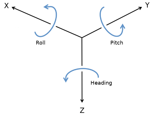
Attitude is our measurement of orientation and is composed of roll, pitch, and heading. Roll is the rotation about X, pitch the rotation about Y, and heading the rotation about Z. Heading is also known as yaw
Together, position and attitude tell us where our robot is and how it is oriented in the earth frame.
Sensors
Next we'll review the sensors that make up our inertial navigation system, trying to understand both how they work and their limitations
Accelerometer
The accelerometer is the only "traditional" inertial sensor that gives us a measurement of our position. Unfortunately, it is not a very good one.
To go from acceleration to position we need to integrate twice, which means that any error in our acceleration will increase quadratically over time. Even small errors in acceleration can result in huge errors in position.
acceleration =    a
velocity     =  ∫ a =     a · t
position     = ∫∫ a = ½ · a · t2
Plugging in an accelerometer bias of 0.0196 m/s2 (which is an actual spec from a $20,000 sensor) into the above position calculation, we would could drift 127 kilometers in an hour while sitting on a bench top.
(½) · 0.0196 meters/second2 · 36002 seconds = 127,008 meters
Magnetometer
A magnetometer measures the magnetic field in 3 spatial dimensions. A compass is a single dimension magnetometer, measuring the magnetic field about Z, defining our heading. Heading is our most important measurement underwater because small errors in heading can lead to large errors in position.
The below chart shows where our robot thinks it ended up after traveling in a straight line for 1 kilometer. The black line shows the true path and the other lines show the calculated course given an error in our heading after starting from the same point.
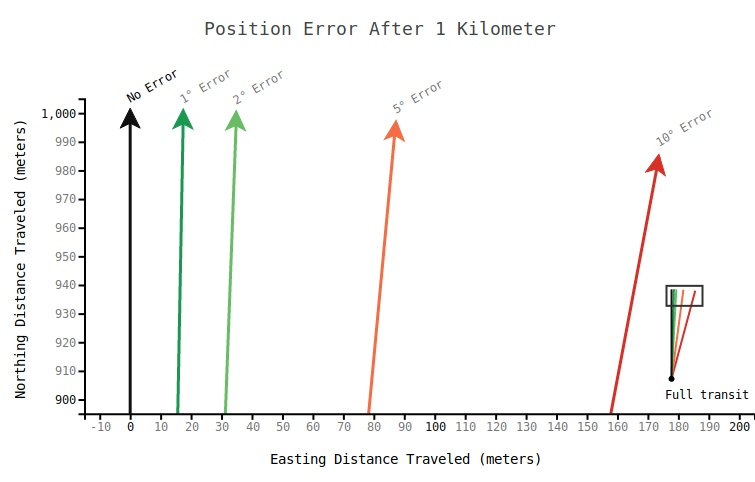
If our heading is off by 10° we'll end up with a position error of 174 meters, which is 17.4% of our distance traveled. 10° might seem like a huge error, but compasses are notoriously fickle, and for good reason. Putting a compass in a metal cage with electricity flowing and whirly bits moving tends to make for unhappy compasses.
We need another sensor to aid in our heading measurement. That’s where the gyroscope comes in.
Gyroscope
While magnetometers measure changes in angular position, gyroscopes measure changes in angular velocity.
Velocity is the first derivative of position, so we need to integrate velocity once in order to get rotational position. The integral of velocity is velocity · time, so our error gets bigger over time, but not nearly as quickly as it does with the accelerometer since we need to integrate twice in that case.
angular velocity =   v
angular position = ∫ v  = v · t
Classic gyroscopes are spinning masses that measure changes in angular momentum. Modern gyroscopes are a bit more sophisticated but are more intuitive to understand. Today’s state-of-the-art gyroscope is the fiber optic gyroscope (FOG) and rather than using conservation of angular momentum, it relies on special relativity to calculate rotational velocity.
Here’s an illustration demonstrating how they work:
Fiber Optic Gyroscope
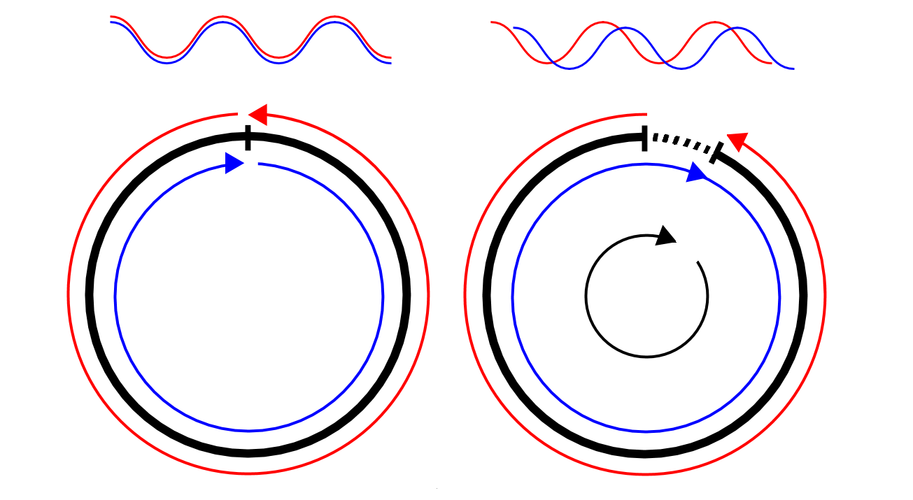
A laser gets shot around a ring in two directions. The image on the left shows a stationary ring (black) with the two beams of the laser (red and blue) arriving back at the origin at the same time. The image on the right shows a ring rotating clockwise. The beam traveling clockwise (blue) has to travel further than the beam traveling counter-clockwise (red) to get back to where it started, resulting in a different interference pattern in a sensor at the origin. This interference pattern is used to derive the angular velocity in the plane of the ring.
FOGs are typically composed of three orthogonal rings and so can measure angular velocity about any axis.
Given that we still need to integrate once to get angular position, gyroscopes will need to be much more precise than magnetometers to outperform them. The good news is that they are. In fact, FOGs are able to measure the rotation of the earth!
The earth rotates 360° in 24 hours, which gives us a rotation rate of 15°/hr. In order to see the full 15°/hr in our heading measurement, we'd need to be at one of the poles. If we were at the equator, we would see no bias from the earth's rotation in our heading measurement (we would see it in roll and/or pitch). The bias due to the rotation of the earth is a function of latitude, so as long as we know our latitude we can factor it out.
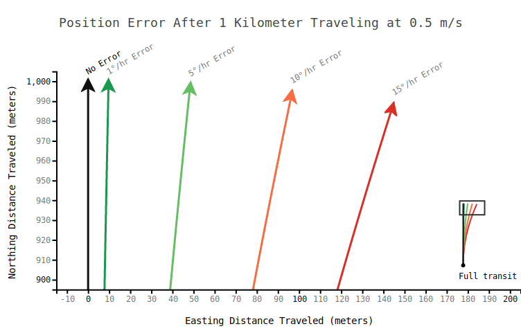
The above plot shows the effect of gyro bias on position error over a 1km run traveling at 0.5 m/s due North. In the above plot, the red line represents the gyro bias due to earth's rotation at the poles. The latitude bias due to the earth's rotation where I live, in Vermont, is about 10°/hr. For FOGs we can expect gyro biases of less than 1°/hr, provided we've factored out the rotation of the earth.
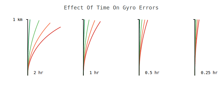
Since we need to integrate rotational velocity to get heading, the error introduced by the gyroscope increases over time. The above plots show the position errors over a 1 kilometer transit for the same biases over different durations. After some amount of time, the error will be worse than the magnetometer error if uncorrected. In practice we are able to combine measurements from the magnetometer and aiding sensors to keep this error in check.
Doppler Velocity Log (DVL)
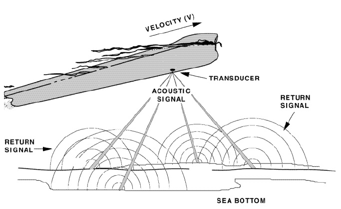
In marine robotics, we are often operating at or near the bottom. When this is the case we can use a DVL to tell us how fast and in what direction we are moving by bouncing sound waves off of the bottom.
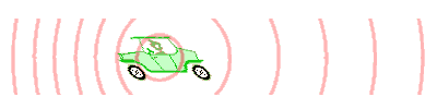
As the name indicates, the Doppler Velocity Log makes measurements utilizing the Doppler shift. The Doppler shift is demonstrated by the animation below. The gist is that given a wave of constant frequency, you’ll experience the wave at a higher frequency when you’re moving toward the source compared to when you’re moving away from the source.
Doppler Shift
The DVL operates by sending a 4-beam signal out of a transducer and then listening for the response. It then measures the phase shift across those 4 beams and reports a speed and course-over-ground.
Course-over-ground is another measurement of rotational velocity and a pretty good one. Like the gyroscope it only provides a relative measurement of heading. It can’t tell us which way is north, but it is very valuable in telling us how far we’ve turned.
The DVL along with our gyroscope, are our two most valuable sensors in marine robotics.
Ultra Short Baseline (USBL)
The USBL is another acoustic instrument but it is the only sensor that we'll discuss that is able to provide an absolute position reference while underwater, though it requires a second vessel on the surface to do so.
A USBL system involves a transceiver on a ship, which sends out a ping to a remotely-operated-vehicle (ROV). The ROV has a transponder that receives that signal and responds with a signal of its own which is in turn handled by the transceiver back on the ship. This transceiver is composed of a transducer array of at least 3 nodes arranged in a triangle. The ship is able to use the time from initial ping to the time of the response to calculate the distance between ship and ROV and the timing difference between transducers to determine the direction to the ROV. This data combined with the GPS position of the ship gives an ROV pilot the position of the vehicle.
GPS
Though we don’t have GPS while we’re underwater, it is still an important aiding sensor. Most vehicles have a GPS on top so that when they’re on the surface they can get an absolute position fix. When the vehicle submerges it must calculate its relative position from this absolute reference to give it an idea of its absolute position in the world.
Handling Sensor Data
So far I’ve described most of the navigation sensors in a typical ROV, but the challenge for the roboticist comes in combining all of that data to get the most accurate solution possible.
The astute observer might have noticed that we could easily factor out the errors discussed above. Given a 10° error in heading we could just subtract 10° from our heading measurement and eliminate our position error. Unfortunately, biases aren't constant over time and are functions of the many changing conditions in our robot.
Noise
We’ve got our suite of sensors but now we need to jam them all together inside of a tiny vehicle with spinning metal, flowing electricity, and other talking sensors. We’ve got acoustic noise (from the DVL, sonar, and USBL), mechanical noise (from motors and spinning parts), electrical noise (from everything), and even temperature effects. Now our expensive sensors with their lovely spec sheets are performing nowhere near how they perform on the bench top.
A large part in designing and maintaining a robotic system involves reducing noise, to the extent that this is possible. This is an art. Characterizing the noise is the first step in the process and iterating on system design to reduce noise is a constant battle. But even the best designed system will have noise.
Fortunately the same mathematical tool that we’ll use to fuse sensor data, also helps us mitigate noise, the Kalman filter.
Kalman Filters
The Kalman filter is the main tool in our toolbelt for taking this disparate and noisy data and turning it into a navigation solution. Kalman filters are an entire subject in themselves and one that I intend to cover in detail in a subsequent post, but this is not that post.
The Kalman filter is a state estimator that allows us to make predictions based on recent measurements and predicted values, resulting in an estimate that is better than either.
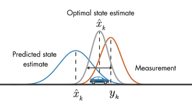
Source: Mathworks
The art of the kalman filter lies in tuning the gains to weight the prediction and measurement terms based on what’s happening in the system.
A simple kalman filter might only include sensor data. If we consider a single degree of freedom, say heading, our measurement is the most direct reading we have of that value, which we get from the magnetometer. Then our prediction is the higher order reading, coming from the gyroscope. In an ideal scenario, the variance from these sensors become the gains of the Kalman filter, though as discussed above there are many sources of noise that we need to account for so this is generally not true in practice.
A more complex Kalman filter would include vehicle control data, such as thruster effort and direction. This data would be incorporated in the prediction. Using vehicle output data can be difficult though. For example, in a strong current we might need to have thrusters spinning just to hold our position. In that case we’d want to penalize the prediction by giving it a higher variance (resulting in a wider curve in the above image). This would bias our state estimate towards our measurement.
In practice, each of the values in our navigation solution might have one or more Kalman filter associated with it.
The Cleverness of Man
Thanks to what Feynman called the "cleverness of man", we are able to arrive at a solution that is surprisingly good, given the challenges of the environment and the limitations of the technology. But even with state-of-the-art sensors and powerful processors, inertial navigation in marine robotics is still a field where advances can be made and proprietary techniques set solutions apart.
I hope you enjoyed this post. If you are interested in more content like this, including an in-depth explanation of kalman filters, you should follow me on twitter or keep an eye my website.
Other Stuff By Matt
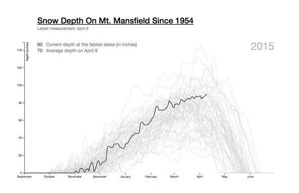
Mt. Mansfield Snow Depth
An interactive graphic that allows users to explore the snow depth on Mt. Mansfield for any season on record. This visualization was retweeted by Edward Tufte (who wrote the book on data visualization) and was shared by the Washington Post on their "Know More" blog.

Lyme On The Rise
A data project for Vermont Public Radio on the growth of Lyme Disease over the last 15 years. Includes an interactive bar graph of New England and small multiples of Vermont and the continental United States showing the infection's expanded range. Published in the open with links to the data.
See the rest - matthewparrilla.com